Simple Linear Regression

Want a straightforward approach to prediction? Nothing is as direct as simple linear regression (SLR). Suppose that you want to predict a quantitative response variable $Y$ on the basis of a single response variable $X$ . It assumes a linear relationship amid the two variables. We say:

$Y \approx \beta_{0}+\beta_{1}X$ [1]

We can think of (1) as the regression of $Y$ on $X$ -this is a surjection. Note that the $\beta_{0}$ and $\beta_{1}$ are two unknown constants that represent the intercept and the slope values in the linear model in (1) -these values, collectively, are known as coefficients or parameters. Once we obtain some data, we can take these values a step further and produce estimators denoted as $\hat{\beta_{0}}$ and $\hat{\beta_{1}}$ . Thus, (1) is now expressed as:

$\hat{y} \approx \hat{\beta_{0}}+\hat{\beta_{1}}x$ [2]

$\hat{y}$ is an estimator for Y based on where X = x. Thus, $\hat{y}$ estimates the values for Y -which is an unknown parameter.

Now that we are this far, we can continue our review with some more pragmatic discussion of how to estimate the values the coefficients. To proceed, we need data; let,

$(x_{1},y_{1}), \ (x_{2},y_{2}), \ (x_{3},y_{3}),...,(x_{n},y_{n})$

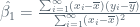
represent n observations (pairs), each of which consists of a measurement of X and a measurement of Y -ultimately, we want to find a line that fits all these observations as close as possible. This idea of closeness is interesting; there are many ways we can define how close we are to the various observations, but the most common (particularly when we are talking about SLR) is least squares criterion

Consider $\hat{y_{i}} \approx \hat{\beta_{0}}+\hat{\beta_{1}}x_{i}$ as the equation that predicts Y based on the $i-th$ value of X. We can no consider the difference amid the value $y_{i}$ and the estimator $\hat{y_{i}}$ which is denoted as the ith residual:

$e_{i} = y_{i}-\hat{y_{i}}$ [4]

Ultimately, (4) will take us to the idea of residual sum of squares and, as we will see, the various coefficients in (2) and (1). The residual sum of squares (RSS) is direct and expressed as:

$RSS = e_{1}^2+e_{2}^2+\dots+e_{n}^2$

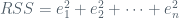
In LSR, we seek to MINIMIZE the RSS. This provides us the values of our coefficients, and hence the linear regression line.

$\hat{\beta_{1}} =\frac{\sum_{i=1}^{\infty} (x_{i}-\overline{x})(y_{i}-\overline{y})}{\sum_{i=1}^{\infty}(x_{i}-\overline{x})^2}$

and

$\hat{\beta_{0}}= \overline{y} - \hat{\beta_{1}}\overline{x}$

With $\frac{1}{n}\sum_{i=1}^{\infty}y_{i}$ and $\frac{1}{n}\sum_{i=1}^{\infty}x_{i}$ as simple means.

Understanding the minimization of RSS is essential, but the concept is not as straightforward as one would think. Infact, it’s easy to understand that $\hat{y_{i}} \approx \hat{\beta_{0}}+\hat{\beta_{1}}x_{i}$ is merely a line in the form $y=mx+b$ with m, and b corresponding to our coefficients. The catch is explaining how the line is formed -how we get the coefficients (its cheap to just place a formula out there) outside the formula.

So, let’s back-up. Our goal is to find a relationship that maps our observations on $x_{i}$ to some y. What does this look like geometrically? There is a great tool here that helps show how this works. If we find a line that does not minimize the RSS, we get something like this:

Screen Shot 2020-04-08 at 12.10.00 PM

The black line is the LSR line, the red line is some other line -note that the red boxes are those that form a square from the point to the red line -the area of those squares is not minimized. That is, we never minimized the RSS to derive the correct values for our coefficients. The black boxes, however, are the areas of the squares of the LSR from each point -notice that they are minimized.

Coefficient Estimates and Accuracy

In general, LSR exhibits high interpretability and low flexibility. There are implications to model selection that must be considered; first, flexible models often require estimating a greater number of parameters and are more complex -this leads to a phenomenon known as overfitting wherein the noise is modeled too closely (the noise is integrated into the model over the signal). Second, there is the quintessential problem of spuriousness that tends to complicate all statistical models -but is more chronic amid problems where highly flexible models are more appropriate (there are methods to dealing with such a problem, but we won’t address that here). Second, there is a tradeoff that takes place amid flexibility and interpretability that is important to consider -as flexibility increases, interpretability tends to decrease.

It is important to highlight that when estimating $\beta_{0}$ and $\beta_{1}$ from our data that there exists a true relationship amid X and Y such that $f(X)=mX+b$ this relationship, however, is one where the error term has mean 0 and is derived from a normal distribution. This relationship is based on the population data. In reality, we rarely have access to such an epistemic vantage point -thus, we are stuck working with a subset of the population data. These observations generate $\hat{y_{i}} \approx \hat{\beta_{0}}+\hat{\beta_{1}}x_{i}$ as a distinct line that is a approximation of $f(X)$ .

Prima facie, the idea of $f(X)$ being different from $\hat{y_{i}}$ is not clear. Why would such a difference exist when we have only one data set to work with? First, this is mora a philosophical actualization and fundamental problem with measurability than anything inherent to the mathematics. Suppose we seek to understand certain characteristics of a large population -suppose further that we want to know the population mean $\mu$ of some random variable Y. We know that we can’t really witness or obtain all the data elements of Y, but we can obtain a sample. This will allow us to estimate the mean of Y. Since we have access to the sample, say n observations from Y; call that k such that $k\subset Y$ , we can find a reasonable estimator $\hat{\mu}$ =\overline{y}$ where $\overline{y}= \frac{1}{n}\sum_{i=1}^{\infty}y_{i}$ as the sample mean. In general, the sample mean is a good estimator for the population mean. Thus, in the same way, the coefficients are being estimated for m and b in $f(X)$ .

The analogy drawn above amid the sample mean and the SLR is apt based on the concept of bias. Think about it…. if we use $\hat{\mu}$ to estimate $\mu$ , the estimate is unbiased on average -so, in some cases the sample mean will overestimate the population mean, and in some cases it will underestimate. However, on average, we expect that, over a huge number of estimates, to equal the value of the population mean. Hence, such an estimator does not systematically fail in estimating the true parameter. This property of unbiasedness holds for:

$\hat{\beta_{1}} =\frac{\sum_{i=1}^{\infty} (x_{i}-\overline{x})(y_{i}-\overline{y})}{\sum_{i=1}^{\infty}(x_{i}-\overline{x})^2}$

and,

$\hat{\beta_{0}}= \overline{y} - \hat{\beta_{1}}\overline{x}$

Now, if we were to average these over a very large number of data sets (pulled from the same population), we would have estimates that are equal to the the “real” coefficients of the population. However, we should be asking ourselves how accurate are these estimators, when unbiased, to the population equivalents. Let’s revert back to our example of the population mean $\mu$ of some random variable Y . So, how accurate is $\hat{\mu}$ as a estimate of $\mu$ ? We have asserted that the average of $\hat{\mu}$ ‘s over many data sets will be very close to $\mu$ -however, a single estimate of $\hat{\mu}$ may substantially underestimate or overestimate $\mu$ How far off could we get? In general, we answer this question by computing the standard error of $\hat{\mu}$ , written as $SE(\hat{\mu})$ We have well-known formula:

$Var(\hat{\mu})=SE(\hat{\mu})^2=\frac{(\sigma^2}{n}$ [5]

Basically, the standard error tells us the average amount that this estimate $\hat{\mu}$ differs from $latex \mu. Take note that where n in (5) is the number of data points, the standard error gets smaller when n gets large -that is, the more observations, the more accurate.

Now, we should be able to obtain an standard error for our coefficients -so, to compute the standard error associated with $\hat{\beta_0}$ and $\hat{\beta_1}$ , we use the following formulas (more details here):

$SE(\hat{\beta_0})^2 = \sigma^2\big[\frac{1}{n} + \frac{\overline{x}^2}{\sum_{i=1}^{\infty} (x_i -\overline{x})^2}$

$SE(\hat{\beta_1})^2 = \frac{\sigma^2}{\sum_{i=1}^{\infty} (x_i -\overline{x})^2}$

where $\sigma^2 =Var(\epsilon)$ . In all these formulas, the demand for them to be valid requires that the error, $\epsilon_i$ , is uncorrelated with common variance $\sigma^2$ Note that we cannot know $\sigma^2$ directly, but we can estimate it; this estimate is known as the residual standard error, and is given by the formula RSE = (RSS/(n-2))^(1/2).

Standard errors are useful for various things; one of these is to compute confidence intervals. A 95% confidence interval (CI) is defined as a 95% probability that a range of values will contain the true unknown value of the parameter in question. The range is defined as upper and lower bounds; the 95% CI for $\beta_1$ is $\hat{\beta_1} \pm 2(SE(\hat{\beta_1})$ which defines the CI:

$\hat{\beta_1} - 2(SE(\hat{\beta_1}), \hat{\beta_1}+ 2(SE(\hat{\beta_1})$

The CI states that there is approximately a 95% confidence interval that our coefficient lies within that interval. We also define the CI for our intercept ( $\beta_0$ ) as $\hat{\beta_0} \pm 2(SE(\hat{\beta_0})$ .

Pulling It All Together

Standard errors are more than just interesting measures to help us understand SLR. We can use these tools to perform hypothesis tests on these coefficients. We proceed as follows (some great resources here):

Formulate a null hypothesis (think of this as the opposite of what you are guessing or looking for in your data).
Provide an alternative hypothesis
Set an $\alpha$ (this involves type 1 and 2 errors – $\alpha$ corresponds to a type 1 error -more on this later)/
Assuming you have correct data, calculate a test statistic (F, T, etc…)
Determine thresholds of rejection.
Derive a decision of fail to reject the null or reject the null.

M	T	W	T	F	S	S
		1	2	3	4	5
6	7	8	9	10	11	12
13	14	15	16	17	18	19
20	21	22	23	24	25	26
27	28	29	30

John Piccolo

"…..no firm demonstration can be made from the success of hypotheses." -G.W. Leibniz

Simple Linear Regression

Coefficient Estimates and Accuracy

Pulling It All Together

Leave a Reply Cancel reply

Coefficient Estimates and Accuracy

Pulling It All Together

Share this:

Like this:

Related

Leave a Reply Cancel reply